
How to apply k-sum optimization on divergent ESG ratings
Handling differing ESG ratings with a novel technique

We have previously talked about the issues of divergent ESG ratings in sustainable investing here and here. Given that this is a feature of ESG investing, researchers have come up with methodologies (such as this) to incorporate these differing ratings in the portfolio optimization process.
This week, we look at a paper titled Managing ESG Ratings Disagreement in Sustainable Portfolio Selection by Francesco Cesarone, Manuel Luis Martino, Federica Ricca and Andrea Scozzari, which applies a novel technique known as k-sum optimization strategy.
To be honest, I have not heard of this before reading this paper, so it is something new for me as well. For a brief introduction of what it is, check out this video:
If I understand correctly, the k-sum optimization strategy aims to find the right combination of k numbers from a given set of numbers whose sum meets a pre-determined criterion.
In our use case, where we have different ESG rating providers, it would mean selecting the optimal set of ratings that yields the best (or avoid the worst) overall portfolio ratings.
Let’s begin!

Divergent ESG Ratings
In the paper, the authors use data from these different rating providers:
Refinitiv ESG Score: 0-100; higher is better
Bloomberg ESG Disclosure Score: 0-100; higher is better
Morningstar Analytics ESG Risk S</a> on <a href="https://unsplash.com/photos/yellow-red-blue-and-green-lego-blocks-kn-UmDZQDjM?utm_content=creditCopyText&utm_medium=referral&utm_source=unsplash">core: 0-100; lower is better
S&P Global ESG Global Rank: 0-100; higher is better
ESG ratings from different providers suffer from the issue of varying evaluations for the same asset due to differences in methodology, which is unavoidable.
This can be likened to an Olympic diving competition where each judge gives a different score, despite looking for the same set of principles.
In the ESG context, the complexity is further increased by the absence of an agreed-upon rulebook to assess companies' ESG efforts.
Therefore, in the first step to ensure ESG evaluations by different providers are coherent, a feature scaling is performed:
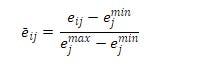
Where i represent the rating agency and j represent a particular stock or company.
The authors then perform analysis on stocks in two indices: NASDAQ100 and EuroStoxx50. The figure below shows the pairwise distances between ESG scores assigned by different agencies for each asset in Nasdaq 100.

For instance, looking at the consistent shade of blue across the first line, we can observe BMG (Bloomberg) and RFT (Refinitiv) are quite close in terms of ratings agreement, but MNG (Morningstar) and S&P have more disagreements, represented by the shades of yellow.
A similar figure but for EuroStoxx 50:

Looking at the summarized metrics measured by various distance scores below, it seems like there is less disagreement in Nasdaq100 compared to EuroStoxx50.
Performing k-sum optimization
According to the authors, k-sum optimization is a more effective technique when markets are characterized by more intense disagreement:
A k-sum optimization approach is used to mitigate the effects of data uncertainty in robust optimization.
One of the key steps in this process would be to convert the ESG score into its complement (1 – ESG score), which we can minimize in our objective function.
In this paper, we have four rating agencies. In the optimization formula used by the authors, a parameter to consider is k, which is the number of rating agencies that we should consider in our optimization.
If k = 1, we find a portfolio that minimizes the worst score for each asset from each agency (not the same agency for the whole portfolio).
If k = 4, our end-portfolio will consider scores from all rating agencies, and will select a configuration that yields the minimum sum of worst-scores.
So when 1 < k < 4, we consider the scores from more than one agency, but not all, agencies.
Incorporating risk-return objective
We have also written previously about incorporating ESG views in a mean-variance framework (here and here).
In this paper, the authors apply this approach but use the k-sum optimization strategy mentioned above to handle divergent ESG ratings.
Without getting too technical, here is the set-up. The authors created four scenarios with increasing level of target returns (µ), based on this formula µ = µmin + α(µmax − µmin), where α = 0, ¼, ½, ¾.
Here is the efficient surface for different levels of target returns:
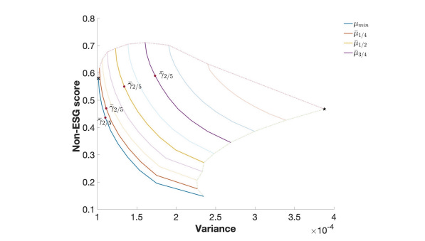
In this diagram, the purple line represents the highest target-return portfolio, followed by yellow, orange and blue. Why this is called a surface instead of a frontier is because there are now three dimensions to consider, instead of the usual two in classical portfolio optimization (risk and return).
Here, ESG rating is the third dimension (represented by its complement term, non-ESG score on the y-axis) and as we fix the target return level based on expected returns, we could derive efficient portfolios that optimize based on an investor’s trade-off between these three components (non-ESG score, expected returns and risk).
Improving one dimension invariably means trading off on one of the other.
For example, look at the purple line above, which has the highest expected return, for the same level of variance we would essentially end up with a higher non-ESG score (since this is the complement, that means a portfolio with worse ESG characteristic).
You may also notice the four dots highlighted above. These are the arbitraily chosen efficient portfolio for performance comparison purpose later on.
For each of the targeted return level, we select the portfolio with an intermediate sustainability value, using a similar formula: γ = γmin + 2/5 (γmax − γmin). The 2/5 is an arbitrary value and used just so we can compare portfolio results.
Empirical results
With the above, the authors then compare results for the various portfolio optimization approaches highlighted below:
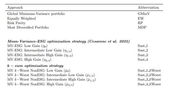
Just to recap, the first four rows (GMinV, EW, RP, MDP) represent classic portfolio optimzation without ESG consideration.
The next four rows, Sust_1 to Sust_4, consider ESG as a third dimension but do not use the k-sum optimization technique.
The last four rows use k-sum with an increasing level of target return (i.e. the dots from the purple, yellow, orange and blue lines in the efficient surface).
The result?
In general, expected returns and Sharpe ratios are better for the three-objective models that incorporate ESG models and have high target returns (Sust_4 and Sust_4_kWorst) compared to standard methods like GMinV, EW, RP and MDP.
Comparing the two ESG optimization strategies, k-sum optimization strategy generally performed better than the standard mean-variance ESG optimization strategy. This suggests that using k-sum may be a better technique in handling disagreement between various ESG vendors.
Drilling into the k-sum optimization strategy, the authors also observe that in general, setting k=3 yields the most optimal result. This “supports the idea that when there is disagreement in the ESG ratings, including the evaluation of more than one agency provides an effective tool for improving the performance of the selected portfolio”.
Summary
So, what have we learned? This is arguably quite a technical paper so kudos for reading till the end.
In short, there are a few useful lessons here, especially on incorporating varying ESG ratings in portfolio optimization:
Including sustainability metrics in the classical mean-variance optimization — essentially turning it into a three-objective optimization model — could yield better results, especially as we target higher expected returns.
When dealing with noisy ESG information from multiple agencies, methods such as k-sum optimization can be a better option. K-sum optimization can exploit all the available information on the ESG evaluation, but, if necessary, it can also select only a subset of ratings to be included in the analysis.
As always, the link to the paper is here if you want to dive deeper.